Signal models
SystemLab|Design uses port, signal and signal link objects to model data flows between functional blocks. Each port is assigned one signal object and can be interconnected to another compatible port through a signal link. The data associated with a signal is held within a Python list. When multiple ports are present, either entering or leaving a functional block, the data is held within a list of lists, for example:
signal_data_list = [[signal_port_a], [signal_port_b],...]
These signal lists are passed as arguments between the functional block data model and the functional block script module. Each data element is accessed as follows:
data_element_1 = signal_data_list[i][j]
# where i is the list index and j is the element index for list i
SystemLab|Design 20.01 provides support for optical, electrical, digital and generic analog signal types. A description of each data model follows.
Optical signal
The optical signal type can be used to represent an optical analog signal (continuously varying with time) that is either guided (e.g. fiber or waveguide confined) or un-guided (free space - geometric). To model the optical signal in a simulation environment, the slowly varying envelope approximation is used [Ref 1]:
where k and w are the wave number and angular frequency of the optical carrier, and Eo is the complex field envelope of the forward propagating wave (which is assumed to be slowly varying compared to the optical carrier wavelength cycle). The complex envelope of the electric field can be represented in either a single array, Exy, or a two dimensional array, Ex and Ey.
The data structure of the optical signal is comprised of data common to all wavelength channels (such as port ID, time samples, and power spectral density) and an optical group list (the collection of optical channels or wavelengths that is linked to the optical signal port):
optical_signal = [portID, sig_type, fs, time_array, psd_array, optical group]

# portID (int): integer ID of the port that is linked to the optical signal
# sig_type (string): The signal type, identified by 'Optical'
# fs (float): The sampling frequency used to capture the sampled signal data
# time_array (1D array): Time samples for the signal
# psd_array (2D array-freq points,psd_points): Optical noise groups (wide bandwidth)
# optical group: The list of optical channels

# Example of two channel optical group:
channel_1 = [wave_key_1, wave_freq_1, jones_vector_1, e_field_array_1, noise_array_1]
channel_2 = [wave_key_2, wave_freq_2, jones_vector_2, e_field_array_2, noise_array_2]
optical_group = [channel_1, channel_2]

# wave_key (int): Wavelength channel key
# wave_freq (float): Frequency of the optical carrier (THz)
# jones_vector: Polarization state data for the electric field
# e_field_array (1D or 2D array): Complex envelope of the the electric field (Eo)
# noise_array (1D array): Time-domain noise values (narrow bandwidth - centered @ optical freq)
An example of an optical signal output for a continuous wave laser is shown in Fig 1. The noise resulting from relative intensity noise (RIN) is shown in red (obtained from noise_array), the field envelope (power - dBm) is shown in blue (obtained from e_field_array), and the frequency domain noise groups (obtained from psd_array) are shown in orange. The frequency domain noise groups can be defined over any optical bandwidth and can be sub-divided into any number of sections (each representing a power spectral noise value for its bandwidth section).
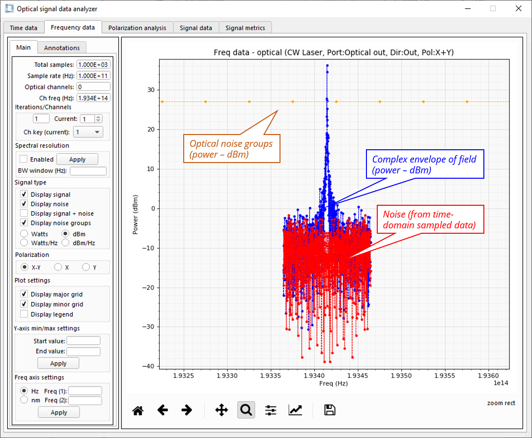
Fig 1: Example frequency domain view for a continuous wave optical laser.
Electrical signal
The electrical signal type can be used to represent an electrical analog signal (continuously varying with time) in the form of either a current or voltage. It can also be used to model free space propagation but only as a scalar appromixation (loss, temporal fluctuations, etc.).
The data structure of the electrical signal is as follows:
electrical_signal = [portID, sig_type, carrier, fs, time_array, sig_array, noise_array]

# portID (int): integer ID of the port that is linked to the electrical signal
# sig_type (string): The signal type, identified by 'Electrical'
# carrier (float): This optional parameter can be used to save a carrier frequency value
# fs (float): The sampling frequency used to capture the sampled signal data
# time_array (1D array): Time samples for the signal
# sig_array (1D array): Sampled amplitude values (real or complex)
# noise_array (1D array): Sampled noise values (real or complex)
Digital signal
The digital signal type can be used to represent a discrete time signal, or a signal that maintains a set value over a given time period. A common example is the binary digital signal which holds a value of 1 or 0 over a specified time period (also called bit period). Multi-level digital signals can also be modeled (for example when analog signals are discretized by analog-to-digital convertors).
The data structure of the digital signal is as follows:
digital_signal = [portID, sig_type, symbol_rate, bit_rate, order, time_array, dig_array]

# portID (int): integer ID of the port that is linked to the digital signal
# sig_type (string): The signal type, identified by 'Digital'
# symbol_rate (float): Symbol rate rate of the signal
# bit_rate (float): Bit rate of the signal
# order (int): Ratio of bit rate to the symbol rate
# time_array (1D array): Time samples for the signal
# dig_array (1D array): Sampled amplitude values of the discrete signal (real)
Analog (1-3) signals
The analog (1), analog (2), and analog (3) signals can be used to represent any kind of analog signal (continuously varying with time); including temperature, pressure, force, sound, etc.
The data structure of the analog signal is as follows:
analog_signal = [portID, signal_type, fs, time_array, amplitude_array]

# portID (int): integer ID of the port that is linked to the analog signal
# sig_type (string): The signal type, identified by 'Analog (1)', 'Analog (2)' or 'Analog (3)'
# fs (float): The sampling frequency used to capture the sampled signal data
# time_array (1D array): Time samples for the signal
# amplitude_array (1D array): Sampled amplitude values of the signal
References
[1] Wikipedia contributors, “Slowly varying envelope approximation,” Wikipedia, The Free Encyclopedia, https://en.wikipedia.org/w/index.php?title=Slowly_varying_envelope_approximation&oldid=871400462 (accessed April 3, 2019).