How to add a customized graph to a design project
In the following tutorial, we will add a customized graph to a laser & optical amplifier model.
Note
A completed version of this design can be found within the folder “systemlab_design\systemlab_examples\optical\optical_amplification"
Part 1: Build the design project “Optical amplification”
Launch a new application of SystemLab|Design by double left-clicking on the SystemLab-Design.exe executable file.
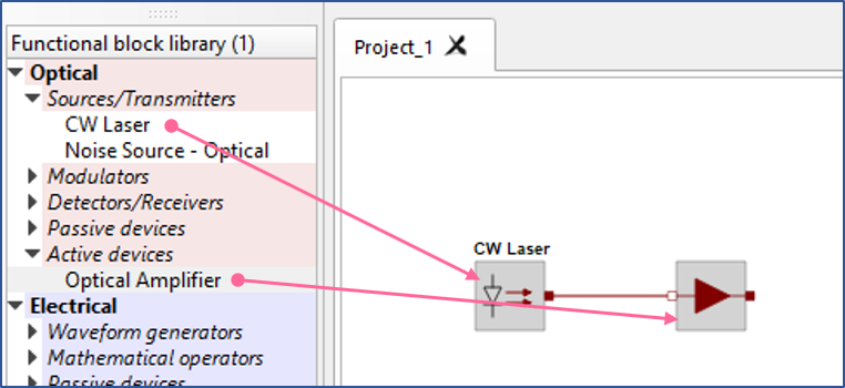
Drag and drop onto the project design space (“Project_1”) a CW Laser and an Optical Amplifier and connect the CW Laser output port to the Optical Amplifier input port as follows:
Before saving the project, navigate to the “systemlab_design” main folder and create a new folder called “optical_amplification”.
Open the Project settings for the design and enter into the Project name field the name “Optical amplification”.
Within the File path (project) field enter the following file path: “.\optical_amplification" and select OK to save and close the Project settings dialog.
Click on the Save icon to save the project file to the new location.
Part 2: Create a project file for the “Optical amplification” design
Open a session of SciTE by selecting Open Python code/script editor from the Menu bar.
Insert the following lines of code at the top of the blank document “1 Untitled” :
#Project file for optical amplification

#Graph for gain vs. input power
amplifier_analyzer = None #Global instantiation for IterationsAnalyzer class
amp_input_power_dbm = None
gain_db = None
Select File/save as from the Menu bar, navigate to the folder “systemlab_design\optical_amplification", and save the project file as: “project_amplifier.py” (Make sure to add the suffix “.py” to the file name!)
Close the file “project_amplifier.py”
Part 3: Create a new QDialog graphing class within “systemlab_viewers”
From the Menu bar select Edit/Custom viewers/graph utilities file/Edit.
Below the class definition for IterationsAnalyzer_NewtonCooling insert the following lines of code [Note: If the class definition for IterationsAnalyzer_Optical_Amp is already present in the code, skip steps 12-15]
class IterationsAnalyzer_Opt_Amp(QtWidgets.QDialog, Ui_Iterations_Analysis):
    '''
    Tab objects (QWidget) are named "tab_xy", "tab_xy_2", etc.
    Graph frame objects (QFrame) are named "graphFrame". "graphFrame_2", etc.
    '''
                def __init__(self, data_x_1, data_y_1):
                        QtWidgets.QDialog.__init__(self)
                        Ui_Iterations_Analysis.__init__(self)
                        self.setupUi(self)
                        syslab_icon = set_icon_window()
                        self.setWindowIcon(syslab_icon)
                        self.setWindowFlags(self.windowFlags()|QtCore.Qt.WindowMinimizeButtonHint)
                        self.iteration = 1
                        self.data_x_1 = data_x_1
                        self.data_y_1 = data_y_1

                        #Setup background colors for frames
                        p = self.graphFrame.palette()
                        p.setColor(self.graphFrame.backgroundRole(), QtGui.QColor(252,252,252))
                        self.graphFrame.setPalette(p)
                        p2 = self.graphFrame_2.palette()
                        p2.setColor(self.graphFrame_2.backgroundRole(), QtGui.QColor(252,252,252))
                        self.graphFrame_2.setPalette(p2)

                        #Setup matplotlib figures and toolbars
                        self.graphLayout = QtWidgets.QVBoxLayout()
                        self.figure = plt.figure()
                        self.canvas = FigureCanvas(self.figure)
                        self.toolbar = NavigationToolbar(self.canvas, self.tab_xy)
                        self.graphLayout.addWidget(self.canvas)
                        self.graphLayout.addWidget(self.toolbar)
                        self.graphFrame.setLayout(self.graphLayout)

                        self.tabData.setCurrentWidget(self.tab_xy)
                        self.tabData.setTabText(0, 'Optical amplifier characteristics')

                        self.figure.tight_layout(pad=0.5, h_pad = 0.8)
                        self.figure.set_tight_layout(True)
                        self.plot_xy()
                        self.canvas.draw()

                def plot_xy(self):
                        ax = self.figure.add_subplot(111, facecolor = '#f9f9f9')
                        ax.clear()
                        ax.plot(self.data_x_1, self.data_y_1, color = 'blue', linestyle = '--',
                                                linewidth= 0.8, marker = 'o', markersize = 3)

                        ax.set_title('Amplifier Gain (small signal)')
                        ax.set_xlabel('Input signal power (dBm)')
                        ax.set_ylabel('Gain (dB)')
                        ax.set_aspect('auto')
                        ax.grid(True)
                        ax.grid(which='major', linestyle=':', linewidth=0.5, color='gray')
                        ax.minorticks_on()
                        ax.grid(which='minor', linestyle=':', linewidth=0.5, color='lightGray')

        '''Close event====================================================================='''
                def closeEvent(self, event):
                        plt.close(self.figure)
Save the changes and close the file “systemlab_viewers.py”.
Close the session of the SciTE editor.
From the Menu bar select Edit/Custom viewers/graph utilities file/Reload. [This will ensure that the Custom viewers/graph utilities file is re-imported into the SystemLab-Design application. If a loading error is raised a warning message will appear outlining the reason for the loading error]
Part 4: Update the “CW Laser” and “Optical Amplifier” scripts
Double left-click on CW Laser to open its Functional block properties.
Select the Edit script icon (next to Script module name) to view the script for “Laser_Source”.
Select File/save as from the Menu bar , navigate to the folder “systemlab_design\optical_amplification", and save the project file as: “Laser_Source_Amp.py” (Make sure to add the suffix “.py” to the file name)
Below Line 12 (from scipy import constants) insert the following lines of code:
#import project_amp
import project_amplifier as project
After line 76 ( time_array = np.linspace(0, time, n) ), add the following three lines of code:
start_pwr_dbm = -20
laser_pwr_dbm = start_pwr_dbm + iteration*0.5
optical_pwr = np.power(10, laser_pwr_dbm /10)
Below the “RESULTS” section (lines 149-159) insert the following lines of code:
'''=DATA LIST FOR GRAPHING==========================================='''

if iteration == 1:
    # First iteration - clear the contents of the input_power_dbm list
    project.amp_input_power_dbm = []
# List is updated with input pwr value over each iteration
project.amp_input_power_dbm.append(laser_pwr_dbm)
Save the changes and close the file “Laser_Source_Amp.py”.
Close the session of the SciTE editor.
Double left-click on Optical Amplifier to open its Functional block properties.
Select the Edit script icon (next to Script module name) to view the script for “Optical_Amplifier”.
Select File/save as from the Menu bar , navigate to the folder “systemlab_design\optical_amplification", and save the project file as: “Optical_Amplifier_Amp.py” (Make sure to add the suffix “.py” to the file name)
Below Line 14 (from scipy import constants) insert the following lines of code:
#import project_amplifier and systemlab_viewers
import project_amplifier as project
import importlib
custom_viewers_path = str('syslab_config_files.systemlab_viewers')
view = importlib.import_module(custom_viewers_path)
Below the “RESULTS” section (lines 143-150) insert the following lines of code:
'''=DATA LIST FOR GRAPHING==========================================='''

if iteration == 1:
    # First iteration - clear the contents of the gain_db list
    project.gain_db = []
# List is updated with new gain value over each iteration
project.gain_db.append(gain_db)

if iteration == iterations:
    # Last iteration - instantiate the xy graph and display results
    project.amplifier_analyzer = view.IterationsAnalyzer_Opt_Amp(project.amp_input_power_dbm,
                                                                 project.gain_db)
    project.amplifier_analyzer.show()
Save the changes and close the file “Laser_Source_Amp.py”.
Close the session of the SciTE editor.
Part 5: Setup iterations and run a simulation
Open the Project settings for the design and set the Number of iterations (under the Simulation settings tab) to 30.
Run a simulation by selecting the Start icon
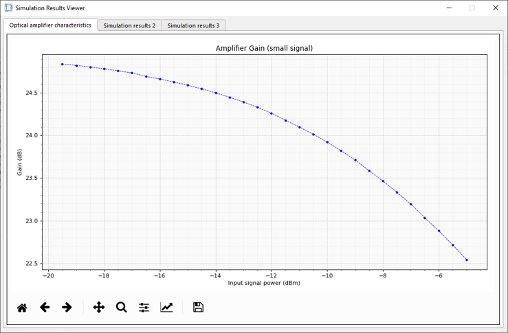
The simulation will run 30 times, each time changing the optical input power level at the amplifier input, and once complete will display a Gain vs Input signal power x-y plot as shown below. As the “Saturated output power” paramter is set to 20 dBm, we can see that the amplifier undegoes gain compression as the output power target (based on the “Small signal gain” setting of 30 dB) exceeds the 20 dBm value. For example at an input power of -8 dBm, the target output should be 23 dBm, but due to saturation the actual gain is around 23.5 (1.5 dB lower).
This completes the tutorial on how to add a customized graph to a design!